Christopher Ferrall
Queen's University
Journal of Statistics Education v.3, n.3 (1995)
Copyright (c) 1995 by Christopher Ferrall, all rights reserved. This text may be freely shared among individuals, but it may not be republished in any medium without express written consent from the author and advance notification of the editor.
Key Words: Teaching aids; Econometrics; Monte Carlo experiments.
This paper discusses a set of programs written in the statistical package Stata that is designed to support interactive student tutorials. The tutorial package has several desirable features, including customized tutorials, full student interaction, checking of student answers, repetition of practice problems using randomly chosen values, and a simple way to gauge student comprehension even when students run the tutorials at home. As an example, a tutorial used in an undergraduate econometrics class is discussed. The example illustrates Monte Carlo experiments on the linear regression model that allow students to demonstrate the validity of various formulas for the sampling distribution of ordinary least squares estimators.
1 There is strong evidence that computer-assisted tutorials can help create an effective environment for learning statistics. In her review of the literature, Garfield (1995) indicates that self-directed learning, feedback on student performance, and reduced computational burden are important elements of statistical tutorials. When applying these lessons to statistics, an effective computer-assisted tutorial should:
1. Be interactive AND statistical. A rich interface must be combined with the capability to perform serious statistical calculations in the background. Since doing statistics necessarily means using a statistical package, the tutorials should teach the material and how to use an underlying statistics package simultaneously. Relying on pedagogical statistical packages means that students must learn (and purchase) other packages in more advanced classes or to complete research projects.
2. Lessen the drudgery of learning statistics. Allow students to enter expressions as answers rather than having to do side calculations. In numerical exercises, provide practice problems that can be repeated with different values that are randomly chosen.
3. Give students feedback on their performance during the tutorial and assess student comprehension after the tutorial.
2 Identifying the features that make computer-assisted tutorials effective learning tools is akin to understanding the demand side of a market. Computer-assisted tutorials must also be effective from the instructional, or supply, side. For instance, tutorial software that requires specialized computer hardware may not be feasible to implement even if it is an excellent teaching tool.
3 Two of the most costly aspects of teaching are coordinated class time and instructor development time. Computer-assisted tutorials can either reduce or increase reliance on these resources. To reduce the demands on computer laboratories and instructor development time, computer-assisted tutorials should have two additional properties:
4. Be tutor-less and independent of specific hardware. If tutorial instructions can be provided electronically, a teaching assistant need not be present, and students can run tutorials in their own time on their own machines.
5. Be programmable. Instructors must be able to customize the material covered in the tutorials as well as share tutorials with other instructors.
4 Roughly one-third to one-half of the students taking my undergraduate econometrics class own computers that can run statistical software. The tutor-less aspect of a tutorial system substantially reduces the burden placed on campus computer capacity. A programmable tutorial system initially entails more development time than a completely "canned" package. However, if the choice is between programming a tutorial and no computer-assisted tutorial that fits the course, then programming may be more attractive. In the long run, programmed tutorials can be shared and built upon so that overall development time falls substantially.
5 This paper describes a system for creating and running statistical tutorials with the imaginative name "Tutor." Tutor is an attempt to implement the desirable features suggested above. An example of a tutorial used in my undergraduate econometrics course, which is one step in a longer tutorial that introduces Monte Carlo experiments, demonstrates features and capabilities of Tutor.
6 Tutor is a set of programs written in the statistical package Stata (compatible with versions 3.0 and higher). Stata has several built-in features that make it possible to program interactive sessions. The programs in Tutor simply make it easier to write interactive tutorials. Tutorials themselves are Stata programs. Some programs may simply display instructions and explanations on the screen. Other programs that make up a tutorial may go through practice problems or allow students to fit data. To write customized tutorials an instructor needs to know enough Stata to replicate the structure of sample tutorials already written.
7 The only requirement for using Tutor is a computer running Stata. Stata runs on most computer platforms, including DOS, Windows, OS/2, Macintosh, and most Unix platforms. An affordable version of DOS and Macintosh Stata called Student Stata maintains all but a few features of the professional version, enabling students to purchase their own copy at a reasonable price. Stata also has structured programming features that make it possible to write interactive programs. Hamilton (1993) is a student manual that accompanies Student Stata. Several other guides and textbooks that use Stata are available.
8 Tutor does not use a graphical interface. From the student point of view, graphical interfaces are usually preferred, but relying on them would make Tutor less portable. As written, Tutor runs on anything from a DOS 286 machine to a Unix workstation.
9 Affordability, portability, and programmability make Stata a good, but certainly not unique, platform for developing tutorial software for a single course. Since the student and professional versions of Stata are fully compatible, students can make a seamless transition from learning statistics with Stata to doing statistics with Stata. From this broader perspective, tutorials written in Stata or other professional packages are preferable to specialized tutorial packages.
10 To a student the command "tutor" looks like any other Stata command. Tutor defines several commands that help students go through the tutorial. Students download the Tutor commands once at the beginning of the term and then download the tutorials as they become available. After entering Stata, a student starts a tutorial (say week5) by simply typing
. tutor week5
11 This loads the programs associated with Tutor and then loads the commands specific to week5. Then an introductory screen is displayed:
  Welcome to ......

            ------------------------------------------------------
            ---------  .       .  ---------  .-------.  .-----.
                |      |       |      |      |       |  |     |
                |      |       |      |      |       |  |-----\
                |      |_______|      |      |_______|  |       \

            ------------------------------------------------------

             A set of programs and interactive tutorials
             in econometrics written and developed by
                     Chris Ferrall
                     Department of Economics
                     Queen's University
                     ferrall@qed.econ.queensu.ca


Press any key to continue.
Do you want to see a summary of available tutor commands (y/n)?. y
Do you want to record what comes to screen in a file (y/n)?. y
12 The second question allows students to store output that comes to the screen in a file so that they do not have to keep notes while going through the tutorial. For instance, one tutorial goes through the elements required to fully describe a hypothesis test. The elements are displayed on a single screen, and examples are given. Students can cut and paste the screen into their homework assignments as a template for reporting their own tests.
13 The summary of Tutor commands look just like a Stata help screen (which it is):
Here are the commands tutor understands:

              . tutor <tutorial name>
              . next
              . goto <number>
              . intro
              . thelp
              . quiz

   tutor   loads the named tutorial, displays its intro screen, goes to step 1
   next    takes you to the next step in the tutorial
   goto    takes you to the step in the tutorial you specify
   intro   re-displays the intro screen for the current tutorial
   thelp   displays this list of commands
   quiz    display the quiz question for this week if there is one.
14 Each of these commands is a simple Stata program which allows a student to navigate through steps in the tutorial. Next, the introduction to the tutorial is displayed (using the Tutor command intro):
                         Tutorial Number 5

         Steps in this Tutorial:
               1. Introduction to Monte Carlo Experiments
               2. Are OLS Estimates Unbiased Under A1-A5?
               3. Specify and Run Your Own OLS Monte Carlo Experiment
               4. List of Questions to Answer Using Monte Carlo
               5. Displays the Currently Loaded OLS Monte Carlo Experiment

 There is a quiz defined for this tutorial.
15 This screen summarizes for the student what the tutorial is going to cover. The tutorial is organized into steps. Each step is a Stata program. Tutorials can be a mix of simple steps that rely on the textbook and Stata manual to teach the mechanics of Stata and complicated steps that demonstrate statistical results interactively or that give the students practice problems.
16 To design a tutorial using Tutor an instructor must
17 Besides the navigation commands that students see, Tutor includes several commands to support the writing of tutorials. Some of the important primitive commands are:
      Command                  Purpose
      -------                  -------
      inprompt <ans> <prompt>  Asks for input with <prompt> and checks against
                               the correct answer <ans>.  (Rounds to two
                               decimal places to allow for approximations and
                               round off.)  Lets the student guess until he/she
                               gets the correct answer or gives up, and pauses
                               to perform Stata commands.  Confirms the answer
                               or provides the correct answer.

      quiz                     Resets the seed of the random number generator
                               using the student's identification number.
                               Calls the program doquiz to display the quiz
                               for the tutorial.

      quizans                  Runs doquiz for each student number, computes
                               the correct answers and stores a table of
                               identification numbers and answers.  (This
                               command is given only to the teaching
                               assistant to check answers submitted by
                               students.)
18 The inprompt command relies on Stata's display command and its request ( ) option. These two elements allow Stata to ask for and display information interactively. Keyboard input is stored as a string in the argument passed to request. The Tutor command inprompt evaluates the input. For example, a step in a tutorial may include the command
inprompt ans "What is the value of the test statistic?"
which displays the prompt and waits for the answer. Students can pause the tutorial to run Stata commands before entering their guesses. Any keyboard input equal to the correct answer will be accepted. For instance, if ans=5, then correct responses include "5" and "10/2" and "mnx/se" if mnx and se are variables with current values 10 and 2. The value in ans may be randomly determined as the student re-runs the tutorial. Inprompt lets the student try to get the correct answer as many times as the student wishes.
19 The quiz command allows the instructor to ask questions whose answers are randomly determined for each student. The correct answer depends upon a number entered by the student; the seed of a pseudo-random number generator is set equal to a function of this input. (I assign a number to each student at the start of the course.) Students are instructed to e-mail their answers to the teaching assistant. The quizans function runs the quiz question for each student number and creates a table of correct values for comparison to the student answers. This system provides a simple means of gauging student comprehension even though students may be running the tutorial completely on their own.
20 These commands help make it easier to write steps of a tutorial. Because a step is itself a program, some steps of specific tutorials have become inherent commands in Tutor. Some of these include:
      xdist   Creates a univariate discrete distribution table
              and asks students to compute selected moments of
              the distribution.

      xydist  Does the same thing as xdist but with a bivariate
              joint distribution.  Independent and non-independent
              distributions are randomly created.

      ztable
      ttable  Displays statistical tables (standard normal and t)
              to the screen.
21 An example of how a tutorial works is Step 3 of the tutorial above. It allows the student to specify and run Monte Carlo experiments on the simple linear regression model:
Y = b1 + b2 * X + u
The student chooses values for b1 and b2, the distribution of u, the sample values of X, the sample size, and the number of Monte Carlo replications. For simplicity, X takes on equally spaced values between LowX and UpX in each sample. Varying LowX and UpX alters the mean and variance of X, and the uniform spacing of X makes it possible to calculate important values such as \sum (X-\barX)*(X-\barX) as functions of LowX, UpX, and N. This in turn makes it possible to inform students of the theoretical distribution of estimators before setting the sample. Students choose the degree of normality in the error term by setting a parameter t where
u ~ N(0,sigma^2) with probability 1 - t, and
u ~ U(-sqrt(3)sigma,sqrt(3)sigma) with probability t.
Here U(a,b) denotes the uniform distribution on the interval (a,b). When t = 0, u is normal. Screen 4 shows how to run the default experiment. (Assumption A.6 is the assumption that the error terms are normally distributed.)
               STEP 3  Specify and Run an OLS Monte Carlo Experiment

See Steps 1 and 2 for explanation and example.

  First you need to set up the parameters of the experiment:

Enter TRUE b1 to use (press ENTER to leave it equal to 1.5).
Enter TRUE b2 term to use (press ENTER to leave equal to -.6).
sigma is the square root of the variance of u.
Enter the TRUE sigma to use (press ENTER to leave equal to 3).
Enter the sample size (press ENTER to leave equal to 15).
Enter number of artificial samples (press ENTER to leave equal to 80).
Enter LOWER bound of X values (press ENTER to leave it equal to -2).
Enter UPPER bound of X values (press ENTER to leave equal to 2).
To satisfy Assumption A.6 enter 0 next or otherwise a number between 0 & 1.
Enter % of u's to be NOT normal (press ENTER to leave equal to 0).
Enter y next if this is the second of two related experiments.
Append results to a previous experiment for comparison (y/n)?.
22 After specifying the experiment the student reviews it before running the simulations.
      You have specified the following Monte Carlo Experiment
          The Currently Loaded OLS Monte Carlo Experiment
          ------------------------------------------------
Population Regression Function:
               Y    =     1.5     +     -.6 * X     +    u

Summary of the PRF:
True beta1                  = 1.5      True beta2                  = -.6
Var(u)                      = 9        % of u's Uniformly Distr.   = 0%
% of u's Normally Distr.    = 100%

Summary of the Sample and the Experimental Design:
sample size (N)             = 15       replications (# of samples) = 80
Smallest X                  = -2       Largest X                   = 2
So in each artificial sample
       X1 = -2.0000     X2 = -1.7140 ...    X15 = 2.0000
Mean of X                   = 0        Sum of X*X                  = 22.857
Sum of (X-meanX)*(X-meanX)  = 22.857
Do you want to run it or not (y/n)?. y
23 The student can see the results of each iteration of the experiment to get a feel for how sampling variation moves the estimated parameters around as the population parameters remain the same. After each iteration the student can choose to stop viewing the results and let the experiment run to completion automatically.
Population Regression Function:
              Y    =     1.5   +   -.6 * X  +   u

Sample Regression Function in Sample #1
              Y    =     2.07    +    -.11  * X   +    e


  Source |       SS       df       MS                  Number of obs =      15
---------+------------------------------               F(  1,    13) =    0.02
   Model |  .256067518     1  .256067518               Prob > F      =  0.8869
Residual |  158.147646    13  12.1652035               R-square      =  0.0016
---------+------------------------------               Adj R-square  = -0.0752
   Total |  158.403713    14   11.314551               Root MSE      =  3.4879

------------------------------------------------------------------------------
       y |      Coef.   Std. Err.       t     P>|t|       [95% Conf. Interval]
---------+--------------------------------------------------------------------
       x |   -.105844   .7295393     -0.145   0.887      -1.681918     1.47023
   _cons |   2.071906   .9005629      2.301   0.039       .1263584    4.017454
------------------------------------------------------------------------------

Notice the difference between the OLS ESTIMATES and the population PARAMETERS.
Press any key to see graph.
24 The graph in Figure 1 shows the the population and sample regression lines and the sample data. Once students are satisfied with what is happening, they can stop looking at each sample and let the experiment run automatically. The results are then loaded and stored as a Stata data set. The student might be asked to demonstrate that the formulas for the variance of the estimated regression coefficients are correct by looking at the sample variation across experiments. The Stata describe and summarize commands display the main features of the experimental data.
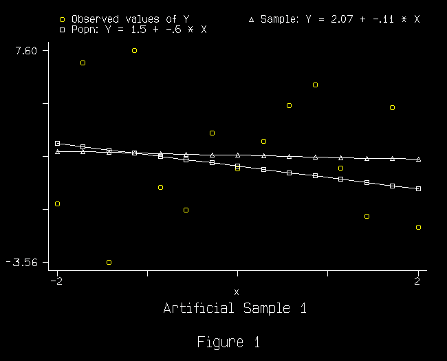 Figure 1. (4K gif)
Figure 1. Monte Carlo Graph.
. describe

Contains data from mmm1.dta
  Obs:    80 (max=   646)                  Monte Carlo Results, N=15
 Vars:     7 (max=    99)
Width:    28 (max=   200)
  1. expno        float  %9.0g             Experiment # (either 1 or 2)
  2. sample       float  %9.0g             sample number
  3. sighat       float  %9.0g             estimate of sigma
  4. b1hat        float  %9.0g             estimate of true_b1
  5. se1          float  %9.0g             estimated standard error of b1h
  6. b2hat        float  %9.0g             estimate of true_b2
  7. se2          float  %9.0g             estimated standard error of b2h
Sorted by:

. summarize

Variable |     Obs        Mean   Std. Dev.       Min        Max
---------+-----------------------------------------------------
   expno |      80           1          0          1          1
  sample |      80        40.5    23.2379          1         80
  sighat |      80    2.851439   .5865814   1.277367   4.358493
   b1hat |      80    1.628286   .7532563  -.1775271   3.810717
     se1 |      80    .7362385   .1514547   .3298146   1.125358
   b2hat |      80   -.5371064   .6468333   -2.19868   .7345619
     se2 |      80    .5964213   .1226923   .2671804   .9116443
25 The true variance of the ordinary least squares estimator of b2 is
Var(u)/\sum(X-\barX)^2 = 9/22.857 = .394.
From the summary table, we can see that the sample standard deviation of b2hat across the 80 samples is 0.647 whose square (0.418) is close to the theoretical variance. Furthermore, the mean value of the estimated standard error of b2hat (0.596) is close to both the actual and theoretical values. Seeing the connection between sampling variation and theoretical formulas is one of the most difficult concepts to understand in statistics. This engine for Monte Carlo experiments and the integrated tutorial program give the students a much better chance of understanding the meaning of the formulas derived in lecture.
26 The quiz for the tutorial containing this step might use the Monte Carlo engine described above to generate experimental results. For example, the quiz could ask the student to determine the proportion of samples in which a 95% confidence interval contains the true value of b1, or it could ask how many times a hypothesis test about b1 is rejected by the data. Students are then led to see directly the correct interpretation of statistical inference.
27 Besides the Monte Carlo exercise, tutorials have been written to demonstrate the central limit theorem, to practice calculating conditional means and variances, to let students visually minimize the sum of squared residuals in a regression, to practice performing hypotheses tests, and to learn how to use the Stata commands required to complete homework assignments such as computing standard errors of forecasts.
28 This paper has discussed Tutor, a program for designing interactive statistical tutorials using Stata. Tutor uses features of Stata to create an interactive environment that can be customized by the instructor. An advantage of Tutor over free-standing educational software is that it is written within the confines of a professional statistical package that students can use beyond their introductory class. Tutor therefore provides continuity between learning and doing statistics.
29 This paper has also argued that instructional software should be evaluated in broad terms. Tutorials and other learning aids should be evaluated for both their learning effectiveness and their cost effectiveness. The high cost of developing and implementing computer-aided tutorials perhaps explains their slow adoption in the light of the evidence that their learning effectiveness can be great. Ultimately, what should emerge is a system for designing tutorials that can be shared with and modified by other teachers so as to lower costs and to pool the talent of many instructors. The tutorial system introduced in this paper is a step in this direction.
I would like to thank Joanne Roberts for her teaching assistance and the students in Economics 351 at Queen's University for their patience, enthusiasm, and pure ability. Tutor and the tutorials used in my class are available by anonymous ftp at highway61.econ.queensu.ca in the directory pub/tutor or through the World Wide Web at http://highway61.econ.queensu.ca/pub/tutor.
Garfield, J. (1995), "How Students Learn Statistics," International Statistical Review, 63(1), 35-48. Also available at http://www.geom.umn.edu/docs/snell/chance/teaching_aids/isi/isi.html
Hamilton, L. C. (1993), Statistics With Stata 3.0, Belmont, CA: Duxbury.
Christopher Ferrall
Department of Economics
Queen's University
Kingston, Ontario K7K 3N6
CANADA
The following Tutor files are needed to run the week5 tutorial.
tutor.readme
tutor.ado
tutor.do
tutor.hlp
week5.do
The file tutor.readme gives instructions for running Tutor.